Variational Auto-Encoders
Deriving ELBO
The goal of a VAE is to learn a latent representation of the data. We do this by mapping the data to a compressed representation, and then reconstructing the data from the compressed representation. An encoder (usually a neural net) $q$ takes a datapoint $x$ as input and outputs the mean $\mu$ and variance $\sigma$ of a Gaussian distribution from which the latent $z$ is sampled. The decoder then reconstructs the data from the latent $z$.
VAEs were introduced in [1] by Kingma et al. Their input distribution consists of binary values instead of real values, and the goal is to maximize the likelihood of the data for generation. Suppose we sampled $z$ from a distribution and then the data $x$ from a distribution conditioned on $z$. The likelihood of the data is then
$$p(x) = \int p(x\,|\,z)p(z)\,dz$$
Maximizing this likelihood using gradient descent is however intractable, so we instead find a lower bound for the likelihood and maximize that. Specifically, we find a lower bound for the log likelihood, which is equivalent. Recall from Bayes' theorem that
$$p(x\,|\,z) = \frac{p(z\,|\,x)p(x)}{p(z)}$$
Now we write the log prob as an expectation over $z$, which lets us do some simplification
$$\begin{align} \log p(x) &= \mathbb{E}_{z \,\sim\, q(z\,|\,x)}\left[\log p(x) \right] \\ &= \mathbb{E}_{z \,\sim\, q(z\,|\,x)}\left[\log{ \frac{p(x\,|\,z)p(z)}{p(z\,|\,x)} \frac{q(z\,|\,x)}{q(z\,|\,x)} }\right] \\ &= \mathbb{E}_{z \,\sim\, q(z\,|\,x)}\left[\log p(x\,|\,z)\right] - \mathbb{E}_{z \,\sim\, q(z\,|\,x)}\left[\log{\frac{q(z\,|\,x)}{p(z)}}\right] + \mathbb{E}_{z \,\sim\, q(z\,|\,x)}\left[\log{ \frac{q(z\,|\,x)}{p(z\,|\,x)} }\right] \\ &= \mathbb{E}_{z \,\sim\, q(z\,|\,x)}\left[\log p(x\,|\,z)\right] - D_{KL}\left(q(z\,|\,x) \,||\, p(z)\right) + D_{KL}\left(q(z\,|\,x) \,||\, p(z\,|\,x)\right) \end{align}$$
Note that the last KL divergence term is intractable because it contains $p(z\,|\,x)$, which is not easy to compute. But since KL divergence is always greater than or equal to zero, we can remove the term and arrive at the lower bound for the log likelihood
$$\log p(x) \geq \mathbb{E}_{z \,\sim\, q(z\,|\,x)}\left[\log p(x\,|\,z)\right] - D_{KL}\left(q(z\,|\,x) \,||\, p(z)\right)$$
which is called the Evidence Lower Bound (ELBO) or the variational lower bound.
Closed-form loss for Gaussian prior
In this case, $p(z) = \mathcal{N}(0, I)$, $q$ (the encoder) will be parametrized by $\phi$, so it'll be $q_{\phi}(z\,|\,x)$, and the decoder will be parametrized by $\theta$, so it'll be $p_{\theta}(x\,|\,z)$. Let's consider the KL divergence term first
$$\begin{align*} D_{KL}(q_{\phi}(z\,|\,x)\,\vert\vert\,p(z)) &= \int q_{\phi}(z\,|\,x)\log{\frac{q_{\phi}(z\,|\,x)}{p(z)}}\,dz \end{align*}$$
Our probability distributions are Gaussians. Given $x$, the encoder will predict the mean $\mu$ and variance $\sigma^2$, so
$$\begin{align*} q_{\phi}(z\,|\,x) &= \mathcal{N}(z\,|\,\mu, \sigma^2) \\ &= \frac{1}{\sqrt{2\pi\sigma^2}}\exp{\left(-\frac{(z - \mu)^2}{2\sigma^2}\right)} \end{align*}$$
The prior $p(z)$ is just the standard Gaussian $\mathcal{N}(0, 1)$ so our KL divergence after substituting becomes
$$D_{KL}(q_{\phi}(z\,|\,x)\,\vert\vert\,p(z)) = \int \frac{1}{\sqrt{2\pi\sigma^2}}\exp{\left(-\frac{(z - \mu)^2}{2\sigma^2}\right)} \log{\frac{\frac{1}{\sqrt{2\pi\sigma^2}}\exp{\left(-\frac{(z - \mu)^2}{2\sigma^2}\right)}} {\frac{1}{\sqrt{2\pi}}\exp(-\frac{z^2}{2})}}\,dz$$
Skipping the long derivation [2] here, but the above simplifies to
$$D_{KL}(q_{\phi}(z\,|\,x)\,\vert\vert\,p(z)) = -\frac{1}{2}\sum_{j=1}^J\left(1 + \log{\sigma_j^2} - \mu_j^2 - \sigma_j^2\right)$$
where $j$ is the mean and variance vector index and $J$ is the dimension of the latent. Now we consider the expected log probability term. The probability is parametrized by $\theta$ since it depends on the mean and standard deviation predicted by the decoder
$$\begin{align*}\log p_{\theta}(x\,|\,z) &= \log{\frac{1}{\sqrt{2\pi \sigma^2}}\exp{\left(-\frac{(x - \mu)^2}{2\sigma^2}\right)}} \\ &= -\frac{1}{2}\log{2\pi\sigma^2} - \frac{(x - \mu)^2}{2\sigma^2} \\ &= -\log{\sigma} - \frac{(x - \mu)^2}{2\sigma^2} \end{align*}$$
where we ignored the constant $\log{2\pi}$. We want the expected log prob though, so we just sample a few $x$s (say, L of them) and take the mean
$$\mathbb{E}_{z \,\sim\, q(z\,|\,x)}\left[\log p_{\theta}(x\,|\,z)\right] \approx \frac{1}{L}\sum_{l=1}^L\left(-\log{\sigma} - \frac{(x_l - \mu)^2}{2\sigma^2}\right)$$
So the objective we're maximizing is
$$\begin{align*} \mathcal{G}(\theta, \phi) &= \mathbb{E}_{z \,\sim\, q(z\,|\,x)}\left[\log p_{\theta}(x\,|\,z)\right] + D_{KL}(q_{\phi}(z\,|\,x)\,\vert\vert\,p(z)) \\ &= \frac{1}{L}\sum_{l=1}^L \sum_{k=1}^K\left(-\log{\sigma_k} - \frac{(x_{l,k} - \mu_k)^2}{2\sigma_k^2}\right) + \frac{1}{2}\sum_{j=1}^J\left(1 + \log{\sigma_j^2} - \mu_j^2 - \sigma_j^2\right) \end{align*}$$
where $K$ is dimension of the output. The loss is just the negative of the above expression (so we minimize it)
$$\mathcal{L}(\theta, \phi) = \frac{1}{L}\sum_{l=1}^L \sum_{k=1}^K\left(\log{\sigma_k} + \frac{(x_{l,k} - \mu_k)^2}{2\sigma_k^2}\right) - \frac{1}{2}\sum_{j=1}^J\left(1 + \log{\sigma_j^2} - \mu_j^2 - \sigma_j^2\right)$$
and this is the loss for a single data point. For a batch, we just take the sum of the losses of each datapoint. As we can see, the expected log prob or the reconstruction loss looks like mean squared error for a Gaussian distribution. We can use other losses as well. If the data is say, normalized images, we can use binary cross-entropy loss instead.
Implementation
Colab notebook here. We'll use MNIST. A simple MLP for the encoder and decoder (up convolution) suffices. A slight modification we do is that the encoder outputs the log variance instead of the variance itself. This is because we want the variance to be always positive and exponentiating the log variance will do that. Let's define the VAE class:
class VAE(nn.Module):
  def __init__(self, zdim):
    super().__init__()
    self.zdim = zdim

    self.encoder = nn.Sequential(
      nn.Linear(784, 256),
      nn.ELU(),
      nn.Linear(256, 64),
      nn.ELU(),
      nn.Linear(64, 32),
      nn.ELU(),
      nn.Linear(32, 2 * zdim)
    )

    self.decoder = nn.Sequential(
      nn.Linear(zdim, 32),
      nn.Linear(32, 64),
      nn.ELU(),
      nn.Linear(64, 256),
      nn.ELU(),
      nn.Linear(256, 784),
      nn.Sigmoid()
    )
This has around 440k parameters. We've used ELU because
ReLU can cause dead neurons. Since we're using
Sigmoid in the output layer, we'll use binary cross-entropy
loss as the reconstruction loss instead of the MSE loss we derived above. We define the
forward pass, where we use the repametrization trick.
def forward(self, x):
  mu, logvar = torch.split(self.encoder(x), self.zdim, dim=1)
  std = (logvar * 0.5).exp()

  # reparametrization trick
  z = std * torch.randn(mu.shape).to(mu.device) + mu

  return self.decoder(z), mu, std, logvar
Why do we use the reparametrization trick? So our network is differentiable. Remember that sampling is not a differentiable operation, so we make use of the fact that $c\sigma(x) = \sigma(cx)$ and $c\mathbb{E}[x] = \mathbb{E}[cx]$ to make the sampling operation differentiable. Now we define the loss function.
def loss(self, x):
  rx, mu, std, logvar = self(x)
  gll = F.binary_cross_entropy(rx, x, reduction='sum')
  kld = -0.5 * (1 + logvar - mu * mu - std * std).sum()
  return gll + kld
As we can see, PyTorch notation is much more concise than the math notation. The training loop is pretty straightforward. We first flatten every MNIST image because we're using an MLP.
device = torch.device('cuda')
batch_size = 128
epochs = 50
lr = 3e-4
zdim = 2

transform = transforms.Compose([
  transforms.ToTensor(),
  transforms.Lambda(lambda x: torch.flatten(x))
])

def train(model, batch_size, lr, epochs):
  loader = torch.utils.data.DataLoader(
    MNIST('.', download=True, transform=transform),
    batch_size=batch_size,
    shuffle=True
  )

  opt = torch.optim.Adam(model.parameters(), lr=lr)

  for epoch in range(1, epochs + 1):
    bar = tqdm(loader, ascii=' >=')
    for x, _ in bar:
      opt.zero_grad()
      loss = model.loss(x.to(device))
      loss.backward()
      opt.step()
      bar.set_postfix({'loss': f'{loss.item():.6f}'})
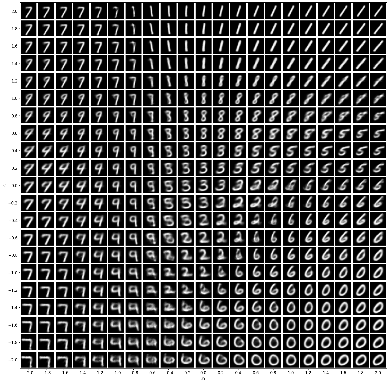
We chose a zdim of 2 so that we can visualize the
latent space easily because every decoder output corresponds to a point in $\mathbb{R}^2$.
Visualizing decoder output for latent vectors in $[-2, 2]^2$ gives us this: