Vanilla policy gradient

Intro

In this post, I'll explain how to implement VPG in Python using PyTorch and OpenAI's gym. We'll teach an agent to play Pong. I'm assuming familiarity with basic RL concepts (watch this video for a revision). Take a look at gym's documentation as well.

Algorithm

The idea behind policy gradient is to increase (or decrease) the probability of actions taken in proportion to returns. $\pi_\theta$ is the policy model parametrized by $\theta$, and $\pi_\theta(s)$ is the probability distribution of actions given the environment state $s$. We need to find $\theta^*$ that maximizes the expected reward objective function

$$J(\theta) = \mathbb{E}_{a \sim \pi_\theta}\Big[G = \sum_{t=0}^T \gamma^t r_{i, t}\Big] = \int_\tau \mathcal{R}(\tau)p_\theta(\tau). \tag{1}$$

$\mathcal{R}(\tau)$ is the return for trajectory $\tau$ (a trajectory or episode is a sequence of state-action-reward tuples $\{(s_0, a_0, r_0),\ldots,(s_{i, T}, a_{i, T}, r_{i, T})\}$) and $p_\theta(\tau)$ is the probability the agent follows trajectory $\tau$. We use gradient ascent to maximize the objective function.

$$\theta \leftarrow \theta + \eta\nabla_\theta J(\theta) \tag{2}$$

where $\eta$ is the learning rate. But how do we compute $\nabla_\theta J(\theta)$? We start with the integral in $(1)$. We use what's called the log trick to simplify

$$\nabla_\theta f(\theta) = f(\theta)\nabla_\theta\log(f(\theta)).$$

Taking gradient on both sides of $(1)$

\begin{eqnarray} \nabla_\theta J(\theta) &=& \nabla_\theta \int_{\tau}\mathcal{R}(\tau)p_\theta(\tau) \\ &=& \int_{\tau}\mathcal{R}(\tau)\nabla_\theta p_\theta(\tau) \\ &=& \int_{\tau}\mathcal{R}(\tau)\nabla_\theta\log (p_\theta(\tau)) p_\theta(\tau) \tag{log trick} \\ &=& \mathbb{E}\Big[\mathcal{R}(\tau)\nabla_\theta\log (p_\theta(\tau))\Big] \\ &\approx& \frac{1}{N}\sum_{i=0}^N \mathcal{R}(\tau_i)\nabla_\theta\log(p_\theta(\tau_i)). \tag{3} \end{eqnarray}

We simplify further. Consider $p_\theta(\tau_i)$ in $(3)$. It's the probability the agent will follow trajectory $\tau_i$, and this probability is dependent on $\theta$. By definition, $\pi_\theta(a \vert s)$ is the probability the agent will take action $a$ in state $s$. Let $P(s' \vert s, a)$ be the probability the environment will transition to state $s'$ given that the agent took action $a$ in state $s$. Then the transition probability of the agent taking action $a$ in state $s$ and moving to state $s'$ is given by $P(s' \vert s, a)\pi_\theta(a \vert s)$. The probability of trajectory $\tau_i$ is the product of all transition probabilities

$$p_\theta(\tau_i) = \prod_{t=0}^{n(\tau_i)} P(s_{i, t + 1} \vert s_{i, t}, a_{i, t})\pi_\theta(a_{i, t} \vert s_{i, t})$$

where $\tau_i$ refers to the $i$th trajectory, and $s_{i, t}$ refers to the state at timestep $t$ of trajectory $i$. Substitute the above in $\nabla_\theta\log(p_\theta(\tau_i))$ in $(3)$

\begin{eqnarray} \nabla_\theta\log(p_\theta(\tau_i)) &=& \nabla_\theta\log\Big(\prod_{t=0}^T P(s_{i, t+1} \vert s_{i, t}, a_{i, t})\pi_\theta(a_{i, t} \vert s_{i, t})\Big) \\ &=& \nabla_\theta\log\Big(\prod_{t=0}^T P(s_{i, t+1} \vert s_{i, t}, a_{i, t})\Big) + \nabla_\theta\log\Big(\prod_{t=0}^T \pi_\theta(a_{i, t} \vert s_{i, t})\Big). \end{eqnarray}

The first term goes away because it is not dependent on $\theta$, so we're left with

\begin{eqnarray} \nabla_\theta\log(p_\theta(\tau_i)) &=& \nabla_\theta\log\Big(\prod_{t=0}^T \pi_\theta(a_{i, t} \vert s_{i, t})\Big) \\ &=& \nabla_\theta\sum_{t=0}^T \log(\pi_\theta(a_{i, t} \vert s_{i, t})). \tag{4} \end{eqnarray}

Substitute $(4)$ in $(3)$, and we get

$$\nabla_\theta J(\theta) = \frac{1}{N} \sum_{i=0}^N \mathcal{R}(\tau_i) \nabla_\theta \sum_{t=0}^{n(\tau_i)} \log(\pi_\theta(a_{i, t} \vert s_{i, t})). \tag{5}$$

This is the policy gradient! The VPG algorithm is as follows.

repeat         
  generate trajectories $\tau_1,\ldots,\tau_N$
  $\theta \leftarrow \theta + \eta\nabla_\theta J(\theta)$  # using (5)
until convergence

Implementation

The algorithm is pretty straightforward to implement. Import the necessary libraries first.

import gym
import sys
import time
import tqdm
import torch
import collections
import numpy as np
import matplotlib.pyplot as plt

We initialize the environment and policy network.

# change env name for different env
env_name = "Pong-v0"
env = gym.make(env_name)
actions = [2, 3]  # custom list or [i for i in range(env.action_space.n)]
prefix = "checkpoints/"  # directory to save logs


# change network architecture for diff env
class net(torch.nn.Module):
  def __init__(self):
    super(net, self).__init__()
    self.fc = torch.nn.Linear(1600, 128)
    self.out = torch.nn.Linear(128, len(actions))

  def forward(self, x):
    x = torch.nn.functional.relu(self.fc(x))
    # always softmax output
    x = torch.nn.functional.softmax(self.out(x), -1)
    return x

Initialize policy network and choose number of frames to pre-process.

pi = net()

frames = 3  # num of consecutive frames to process

If we're training an Atari agent, a single frame may not contain information like velocity, or fire-rate, etc. So the policy network will receive a pre-processed sequence of the previous $k$ frames. We store the previous $k$ frames in a Python collections.deque instance called seq. Here, frames = 3. The frame sequence pre-processing function is as follows.

def phi(seq):
  seq = np.array(seq)
  seq = seq[::2, 34:194, :, 1]
  seq[seq == 72] = 0
  seq[seq != 0] = 1
  seq = seq[1] - seq[0]
  seq = seq[::4, ::4]
  return seq.ravel()

Define helper functions.

# convert input to PyTorch tensor
def tensor(x):
  return torch.as_tensor(x, dtype=torch.float32)
  
# convert probability distribution to logits
def logits(s):
  return torch.distributions.Categorical(pi(s))


# sample an action from probability distribution
def act(s):
  return logits(s).sample().item()


# compute loss or objective J given trajectory (states, actions, and rewards)
def loss(S, A, V):
  logp = logits(S).log_prob(A)
  return -(logp * V).sum()

Look at the VPG pseudocode. We generate trajectories, and compute the objective gradient using them. Let's define a function to generate a trajectory, i.e., an episode, and return the states visited, actions taken, and rewards received.

def tau(render=False):
  done = False
  # states, actions, and rewards
  S, A, R = [], [], []
  s = env.reset()
  # store current (and previous) frame(s)
  seq = collections.deque(
    [np.zeros_like(s)] * (frames - 1) + [s], 
    maxlen=frames
  )
  with torch.no_grad():
    while not done:
      s = phi(seq)  # pre-process frames
      S.append(s)  # store processed
      i = act(tensor(s))  # sample action index
      a = actions[i]  # get action
      s, r, done, _ = env.step(a)  # take action
      seq.append(s)  # append next frame to seq
      A.append(i)  # store action
      R.append(r)  # store reward
      if render:
        env.render()
        time.sleep(1 / 45)
  # close env and return transitions
  env.close()
  return np.array(S), np.array(A), np.array(R)

Finally, we define the main training loop.

def train(epochs, N, mod, gamma, opt):
  losses = []
  rewards = []
  lossesf = open(prefix + f"losses.txt", "w")
  rewardsf = open(prefix + f"rewards.txt", "w")
  # start clock
  start = time.time()
  # train loop
  for epoch in range(1, epochs + 1):
    J = 0  # reward
    r = 0  # avg return for N episodes
    # compute expected reward
    for _ in range(N):
      S, A, R = tau()
      r += R.sum()
      for t in range(len(R) - 2, -1, -1):
        R[t] += gamma * R[t + 1]
      R = (R - R.mean()) / R.std()  # normalize returns
      J += loss(tensor(S), tensor(A), tensor(R))  # compute loss
    # backprop and step
    opt.zero_grad()
    J /= N
    J.backward()
    opt.step()
    # return reward and loss
    rewards.append(r / N)
    losses.append(J.item())
    # boring logging :P
    if epoch % mod == 0:
      print("epoch: {}  reward: {:.3f}  loss: {:.3f}".format(epoch, rewards[-1], losses[-1]))
      lossesf.write(f"{losses[-1]}\n")
      rewardsf.write(f"{rewards[-1]}\n")
      torch.save(pi.state_dict(), prefix + f"{epoch}.pt")
  # end clock
  print("train time: {:.2f}s".format(time.time() - start))
  # return losses and episode
  return losses, rewards

Take a look at my GitHub repo. The library imports and above function and variable definitions are in a file called net.py. In train.py, we import everything from net.py for training. Here, we define the optimizer and hyperparameters.

from net import *


# choose hyperparameters
lr = 2.5e-4
epochs = 600
N = 20  # E[R] ~ sum(pi(a_t | s_t)V_t) / N
mod = 5  # checkpoint once every mod epochs
gamma = 0.99  # reward discount

# initialize optimiser
opt = torch.optim.Adam(pi.parameters(), lr=lr)

Create files to log loss and return from each epoch and train the agent.

lossesf = open(prefix + f"losses.txt", "w")
rewardsf = open(prefix + f"rewards.txt", "w")

# train policy network
losses, rewards = train(epochs, N, mod, gamma, opt)

Plot and save the graphs.

fig = plt.figure(figsize=(8, 8))

x = list(range(1, epochs + 1))

plt.xlabel("epoch")
plt.ylabel("loss")
plt.plot(x, losses)
plt.savefig(prefix + f"losses.png")

plt.clf()

plt.xlabel("epoch")
plt.ylabel("reward")
plt.plot(x, rewards)
plt.savefig(prefix + f"rewards.png")

So, how does the trained agent play Pong?

Untrained

Trained

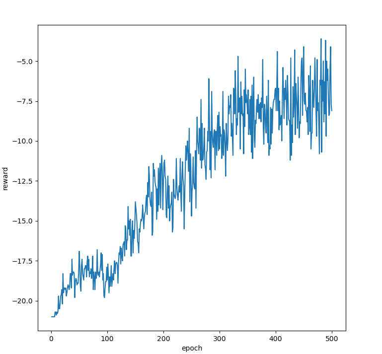
Returns increasing $\implies$ agent learning!

There we go, we have a Pong player.