Deep Q-learning

more posts

Intro

Deep Q-learning is an algorithm introduced by DeepMind in 2015 that kickstarted deep RL. The idea was to combine a traditional RL algorithm (Q-learning) with function approximators, i.e., deep neural nets. In this post, I'll explain the algorithm and how to implement it in PyTorch using OpenAI's gym.

DQL agent playing Atari Breakout

Algorithm

The $Q$ function is the expected discounted return for an agent given that it took action $a$ in state $s$

If we have the optimal $Q$ function $Q^*$ for some RL task, the policy that maximizes the return is to pick the action which yields the maximum return for a given state

Suppose the agent takes action $a$ in state $s$, receives reward $r$, transitions to state $s'$ and takes action $a'$. Then

This relation holds because of the definition of the $Q$ function. If the agent follows the optimal policy, then the action it's going to pick next is that which yields the maximum expected return, i.e., maximum $Q$ value. So the optimal $Q$ function follows the relation

The idea behind deep Q-learning is to approximate the $Q$ function using some model with parameters $\theta$, usually a neural net. The state of the environment is the input and the final layer of the neural net consists of the Q-values for different actions.

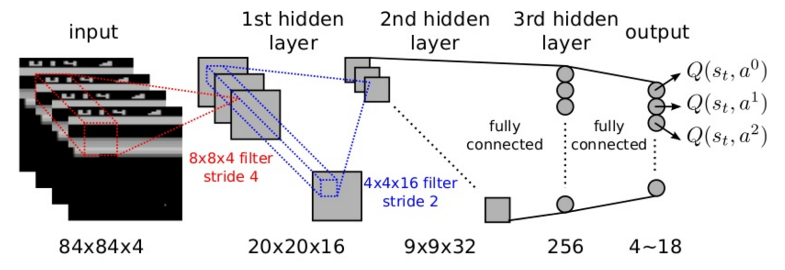
Deep Q-network for playing Atari Breakout

As with all models, $\theta$ is randomly initialized, so $Q_\theta$ doesn't follow any relation. We want to find $\theta$ that satisfies

which is the same relation as $(4)$. How do we find $\theta$ that satisfies the above equation? We use gradient descent. We generate trajectories (or episodes) using an $\epsilon$-greedy policy, i.e., pick a random action with probability $\epsilon$ or choose action with maximum $Q$ value with probability $1-\epsilon$ at each timestep. The transition tuples of the generated trajectory

are added to the replay memory $D$, which is the set of all transition tuples from all trajectories. We sample a bunch of tuples of the form $(s_t, r_t, a_t, s_{t}')$ ($s'$ denotes $s$'s next state) from this memory and tune our model. Let's call this sampled batch $B$

For each tuple in $B$, relation $(5)$ needs to hold up

but it doesn't because $\theta$ was initialized randomly and the model is outputting garbage values. We need LHS to be equal to the RHS above for all transition tuples. Let RHS be the target value $y_i$

and LHS be the prediction. We now have a dataset of predictions and target values. So like supervised learning, we train the model using SGD. The slight difference between supervised learning and RL is that we are generating the dataset by letting the agent follow an $\epsilon$-greedy policy and return the transition tuples from episodes. The pseudocode is as follows.

initialize replay memory $D$
repeat
  # Python deque with k - 1 NULL frames and a start frame
  $S = \{\text{NULL}, \ldots, s\}$ 
  $\psi \leftarrow \phi(S)$  # initial pre-processed sequence
  repeat
    pick action $a$ acc. $e$-greedy and $\psi$
    take action $a$, get reward $r$, and next state $s'$
    append $s'$ to $S$
    $\psi' \leftarrow \phi(S)$
    append $(\psi, a, r, \psi')$ to $D$
    $\psi \leftarrow \psi'$
    sample mini-batch $B \subset D$
    for all $(\psi, a, r, \psi') \in B$
      $
        y\leftarrow 
        \begin{cases}
          r & \psi'\ \text{is terminal} \\
          r + \gamma\operatorname{max}_a Q_\theta(\psi', a) & \text{o/w}
        \end{cases}
      $
      gradient descent step on $(y - Q_\theta(\psi, a))^2$
  until episode done
until convergence

The frame sequence pre-processing is done by storing the last $k$ frames in a collections.deque instance called seq (see implementation below). Initially, we store $k - 1$ numpy array of zeroes of the same dimension as the first state. collections.deque.append deletes first element (i.e., state $s_{t - k + 1}$) and the new element (i.e., state $s_{t + 1}$) is added.

Implementation

Import necessary libraries, define hyperparameters, and initialize Q network and environment.

import gym
import time
import torch
import random
import collections
import numpy as np
import matplotlib.pyplot as plt


# define the Q network
class network(torch.nn.Module):
  def __init__(self):
    super(network, self).__init__()
    # define layers
    self.fc = torch.nn.Linear(4, 256)
    self.out = torch.nn.Linear(256, 2)

  # forward pass
  def forward(self, x):
    x = torch.nn.functional.relu(self.fc(x))
    x = torch.nn.functional.relu(self.out(x))
    return x


# initialize the network
Q = network()

# initialize the environment
e = gym.make("CartPole-v0")

# hyperparameters
N = 100  # episodes
eps = 0.9  # epsilon
# decay epsilon as agent gets better
decay = 0.99
gamma = 0.99999
lr = 1e-3  # learing rate eta
capacity = 2000  # replay memory capacity
# size of sample to take from replay memory
batch_size = 256

# define optimizer
opt = torch.optim.Adam(Q.parameters(), lr=lr)

We define the frame sequence pre-processing function $\phi$.

def phi(s):
    return torch.tensor(s, dtype=torch.float32)

We want to test out our $Q$ network. We define a simple loop to calculate episode return.

def play():
  d = False
  s = e.reset()
  G = 0
  with torch.no_grad():
    while not d:
      s = phi(s)
      a = np.argmax(Q(s)).item()
      s, r, d, _ = e.step(a)
      G += r
  return G

Now we define the training loop as per the pseudocode.

def train():
  global Q, eps, opt
  # intiailize empty replay memory
  D = collections.deque(maxlen=capacity)
  G = []  # store returns
  # main loop
  for i in range(1, N + 1):
    d = False
    s = phi(e.reset())
    # run episode
    while not d:
      # choose action acc. eps-greedy
      if random.random() < eps:
        a = e.action_space.sample()
      else:
        with torch.no_grad():
          a = torch.argmax(Q(s)).item()
      # take action
      ns, r, d, _ = e.step(a)
      ns = phi(ns)
      # store transition in replay memory
      D.append((s, a, r, ns, d))
      s = ns
      # sample batch of transitions from D
      if len(D) <= batch_size:
        B = D
      else:
        B = random.sample(D, batch_size)
      # for each transition in B
      for (s_, a_, r_, ns_, d_) in B:
        opt.zero_grad()
        # compute target
        with torch.no_grad():
          if d_:
            # target val
            y = torch.tensor(r_, dtype=torch.float32) 
          else:
            y = r_ + gamma * torch.max(Q(ns_))
        Qs = Q(s_)  # predicted Q vals
        loss = (y - Qs[a_]) ** 2  # compute loss
        loss.backward()  # backprop
        opt.step()  # update params
    # play a game w/ new Q and store return
    G.append(play())
    eps *= decay  # decay eps
    # log once every 10 episodes
    if i % 10 == 0:
      print(f"episode: {i}\treturn: {G[-1]}")
  # return returns
  return G

Train and save the model and returns plot.

G = train()

# save the trained model
torch.save(Q.state_dict(), "Q.pt")

# plot returns
fig = plt.figure(figsize=(8, 8))
plt.xlabel("episode")
plt.ylabel("return")
plt.plot(np.arange(N), G)
# save plot
plt.savefig("returns.png")

Output should look like so:

episode: 10   return: 9.0
episode: 20   return: 30.0
episode: 30   return: 200.0
episode: 40   return: 200.0
episode: 50   return: 200.0
episode: 60   return: 200.0
episode: 70   return: 200.0
episode: 80   return: 200.0
episode: 90   return: 141.0
episode: 100  return: 105.0

The agent quickly improves.

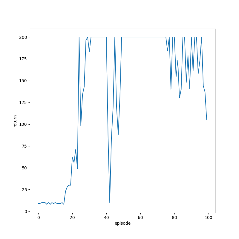
We get the maximum possible return by episode 30.

Agent balancing pole after training.